Rendering Fine Detail with the Distance Estimation Method

In this post we'll learn about the Distance Estimation Method (DEM) which can reveal fine detail not visible with the standard method. We'll also try to understand intuitively what the method is doing, as well as derive the maths behind the algorithm too.

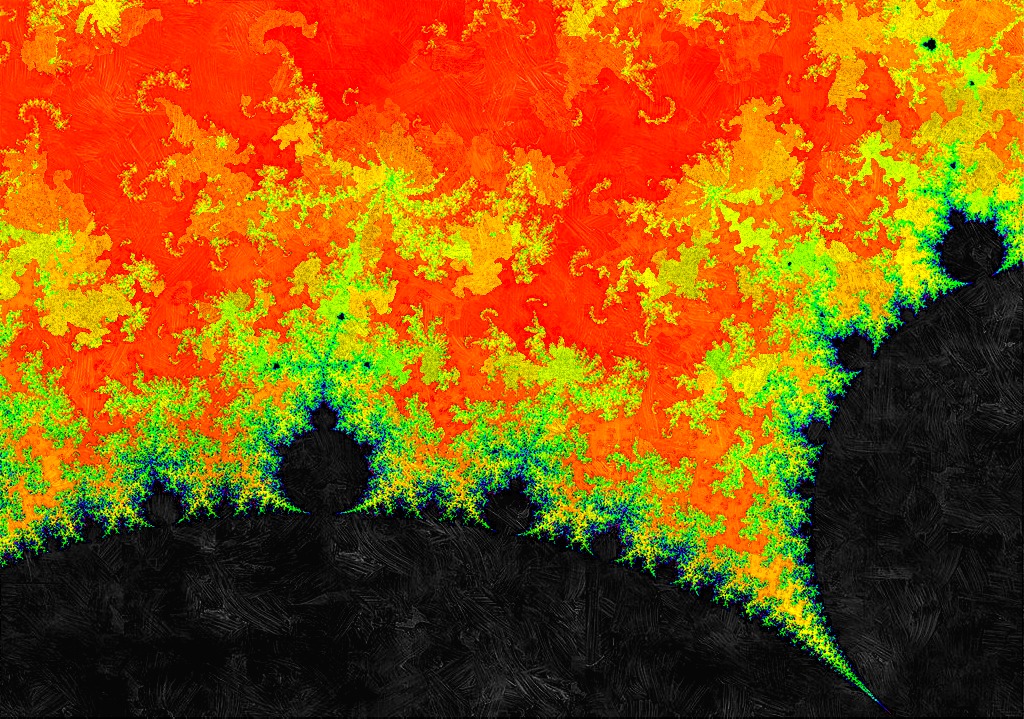
As a taste, the following is a Julia set rendered using the DEM method.

Two Problems

As a reminder, the standard method for rendering Mandelbrot and Julia sets is to repeatedly iterate $z_{n+1} = z_n^2 + c$ and see if the orbit of $z_n$ diverges. 

We can use an escape condition to check for divergence. If $|z_n|>2$ then we can guarantee the orbit of $z_0$ diverges. For Julia sets, the escape condition has two tests, $|z_n| >2$ and $|z|>|c|$.

However, orbits close to, but just outside, the Mandelbrot and Julia set boundaries can take a long time to escape and we can only run the iterations a finite number of times. Similarly, points inside the sets don't diverge, but since we only run a finite number of iterations, we can't be sure they won't escape later.

This makes the standard algorithm for rendering the Mandelbrot and Julia sets imperfect - but generally good enough for most purposes. We trade off accuracy with the maximum number of iterations we test a point for, in effect, the time it takes to complete a rendering.

There is a second problem.

The points on the complex plane that we test correspond to the pixels we want to colour. Those pixels form a grid. The points we actually test are also a grid, usually corresponding with the centre or corner of a pixel. The problem with this is that very fine structure is entirely missed. 

Have a look at the default view of the Mandlebrot. The following shows "blobs" away from the main body. The appear to be disconnected, but we know they are connected to the Mandelbrot set. 

We know that in deep zooms around the edge of the Mandelbrot and Julia sets, there are intricate and quite abundant structures made of very fine structures - filaments - but they are invisible to the standard algorithm because these filaments fall between the grid of points being tested.

Now, we could colour the outside of the Mandelbrot set in an attempt to reveal this hidden structure. The very common "escape speed" method should be appropriate because it colours pixels according to how rapidly they reach the escape criteria. The following shows the same zoomed in region of the Mandelbrot set, on the left without the colouring, and on the right with this escape time colouring.

We can see on the left several "mini-mandelbrot" blobs but not the connecting structure. On the right the colouring has overwhelmed the image making it difficult to see the actual set.

The following shows the same but for a zoomed in region of a Julia set.

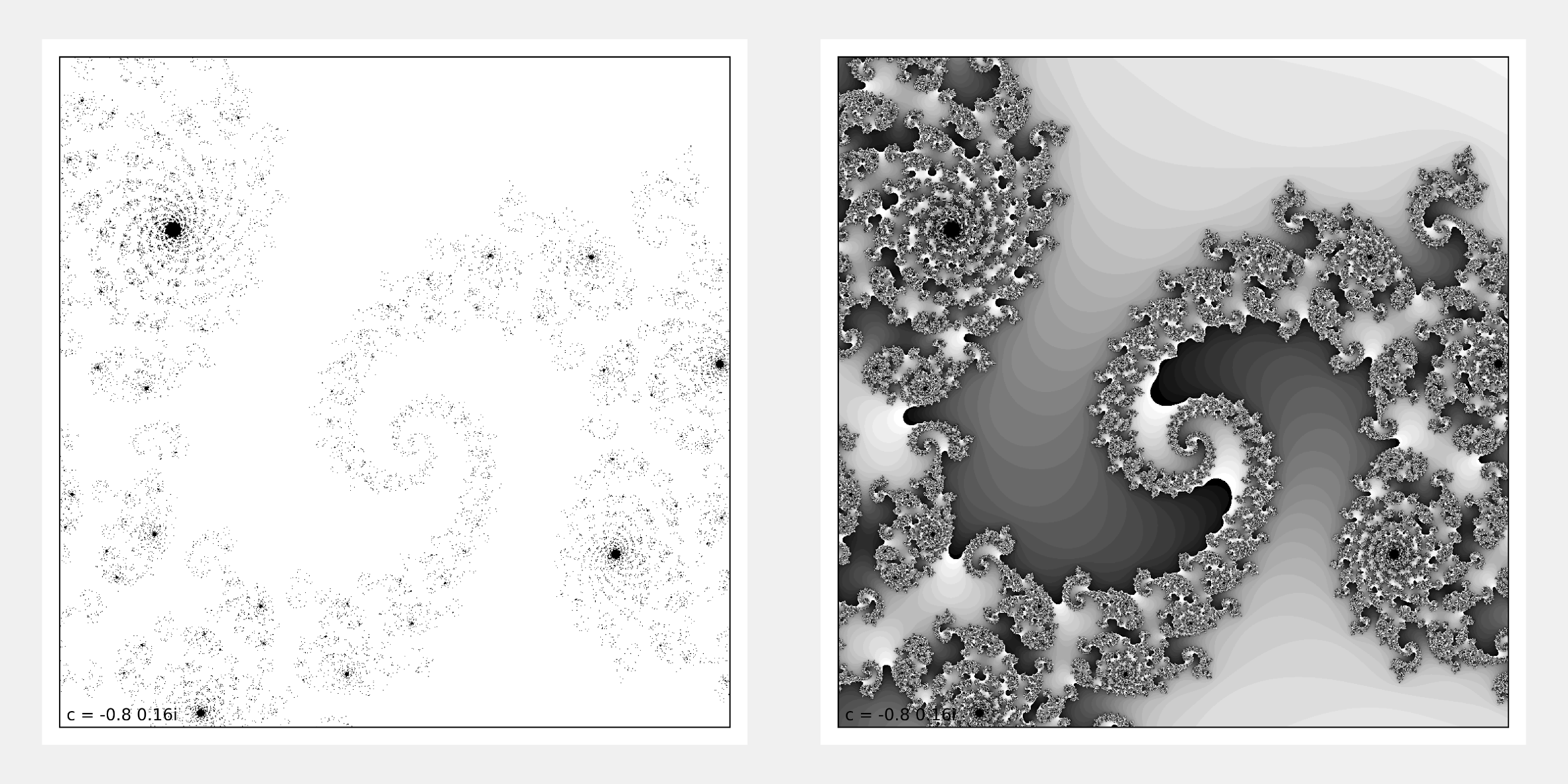
The image on the left is not too bad, but only because the collection of tiny blobs do hint at an intricate structure.

We need a new method.

Distance Estimation (by Gradient) Method

You will have noticed that away from the Mandelbrot and Julia sets, the escape-time coloured regions are larger. Their isolines are more widely spaced out. Closer to the boundary, the regions are thinner,  the isolines are pressed more closely together. The following image highlights these isolines.

If you are familiar with topographic maps, you'll know that altitude (height) isolines close together means a steeper rise or fall,  and widely spaced isolines means a shallow rise or descent. The same is true here.

The gradient of the magnitude of $z$ closer to the edge is higher than the gradient further away from the edge.

This is the key realisation that is behind the Distance Estimation Method. It uses the gradient to estimate the distance from the boundary (any boundary) of the Mandelbrot or Julia sets. 

The benefit of this method is that the points we test, the points that correspond to the grid of pixels, only need to be near the edge of the Mandelbrot or Julia sets to detect that edge. For very fine filaments, again, the points only need to be near them to detect them.

 

Results!

Further below, we'll talk about the algorithm and necessary calculations, but for now let's see how this method improves on the above Mandelbrot and Julia zooms.

The following shows the exact same zoom into the Mandelbrot set as above. The newly revealed structure is very impressive!

The following shows the same zoom into the Julia set as above. Again the resulting detail is amazing.

 

The Algorithm

Before we write down the algorithm, let's first derive how the gradient is calculated.

The primary calculation is the iteration:

$$z_{n+1} = z_n^2 + c$$

For the Mandelbrot set, $z_0=0$ and $c$ is the point being tested. For Julia sets, $c$ is fixed, and $z_0$ is the point being tested.

Now let's work out the gradient (with thanks to Claude for helpful guidance on math stackexchange).

---

For the Julia set, we have fixed $c$ and are testing each $z_0$. Therefore the gradient of $z_n$ is with respect to $z_0$.  

We can differentiate the primary iteration expression using the chain rule, noting that $c$ is constant so its differential is zero.

$$ \frac{d}{dz_0} z_{n+1} = 2 \times z_n \times \frac{d}{dz_0} z_{n} + 0$$

We can write this more simply as

$$z_{n+1}' = 2 z_n  z_n'$$

Whilst this may look unhelpful, this form actually works well with the iterative algorithm. That is, at each iteration:

• as usual, we calculate $z_{n+1}$ from the previous $z_n$ using $z_{n+1} = z_n^2 + c$
• we also calculate $z_{n+1}'$ from the previous $z_n'$ using $z_{n+1}' = 2 z_n  z_n'$

But what should the initial value of the gradient $z_0'$ be set to? Well,

$$z_0' = \frac{dz_0}{dz_0} = 1$$

This tell us to initialise $z_0'$ to 1, in the case of Julia sets.

---

For the Mandelbrot set, we have fixed $z_0 = 0$ and are testing different $c$. Therefore the gradient of $z_n$ is with respect to $c$.

The differentiation is slightly different now.

$$ \frac{d}{dc} z_{n+1} = 2 \times z_n \times \frac{d}{dc} z_{n} + 1$$

We can write this more simply as

$$z_{n+1}' = 2 z_n  z_n' + 1$$ 

Again, what should the initial value of the gradient $z_0'$ be set to? This time,

$$z_0' = \frac{dz_0}{dc} = 0$$

So we initialise $z_0'$ to 0, in the case of the Mandelbrot set.

---

DEM Mandelbrot Set Pseudocode

• or each test point, calculate $c$
• initialise $z_{0}=(0+0i)$
• also initialise the gradient $dz_{0}=(0+0i)$
• for the maximum allowed iterations
• calculate next $z$ using $z\mapsto z^{2}+c$
• calculate next gradient $dz$ using $dz\mapsto2\cdot z\cdot dz+1$
• break out of iteration loop if $|z|>4$ escape condition met
• calculate the distance estimate as $d=\left(|z|\cdot\log|z|\right)/|dz|$
• colour the pixel based on distance estimate, for example $255\times\tanh(d\times\text{resolution}/\text{size})$

Because we're primarily using this technique to explore fine detail, we'll boost the maximum allowed iterations to 4096. We'll also increase the escape radius from 2 to 4, to give the gradient a chance to develop. Both of these will cause the rendering to take longer.

The suggestion for colouring the pixel uses the hyperbolic tangent $\tanh()$ function which squishes all values, no matter how large, into the range 0 to 1, ready for scaling up to 0-255.

Notice that the pixel colour is not based on escape speed, the iterations it took to meet the escape condition, but the distance estimate, which itself is based on the gradient of the orbit of $z$. 

The distance estime $d=\left(|z|\cdot\log|z|\right)/|dz|$ is the only thing we haven't explained here. Your can find out more here. The key is that the larger the gradient the smaller the distance, the rest is scaling.

---

DEM Julia  Set Pseudocode

The algorithm changes slightly for Julia sets.

• $c$ is chosen and fixed
• for each test point, calculate $z_{0}$
• also initialise the gradient $dz_{0}=(1+0i)$
• for the maximum allowed iterations
• calculate next $z$ using $z\mapsto z^{2}+c$
• calculate next gradient $dz$ using $dz\mapsto2\cdot z\cdot dz$
• break out of iteration loop if $|z|>4$ escape condition met
• calculate the distance estimate as $d=\left(|z|\cdot\log|z|\right)/|dz|$
• colour the pixel based on distance estimate, for example $255\times\tanh(d\times\text{resolution}/\text{size})$

Notice the gradient is initialised to 1, not 0, and is updated as $dz\mapsto2\cdot z\cdot dz$, not $dz\mapsto2\cdot z\cdot dz+1$.

Art

The following is a zoom into the Mandelbtot set rendered using this Distance Estimation method.

I love the different shapes and balance of positive and negative space, and also the contrast between the spiral and patterned regions.

I love it so much, I made it the cover image of the Second Edition of Make Your Own Mandelbrot !

Second Edition is out!

 The Second Edition is out - as ebook, paperback and hardback.

This book is written specifically for anyone who is curious about what the famous Mandelbrot Set fractal is, and how to recreate it, but has struggled with the traditional textbooks and online guides.

• Explore what a fractal is, artificial and natural.
• Learn about functions, iteration, and chaos.
• Discover the (not so) complex numbers.
• Find out what the Mandelbrot and Julia Sets really are.
• Follow a hands-on tutorial to make your own Mandelbrot and Julia Sets in python.
• Discover different ways to render the fractals - escape time, image filters, and 3d landscapes.
• Bonus chapter on distance estimation to reveal very fine detail.

 

This book is aimed at complete beginners, and only requires a browser and internet connection to follow the tutorials. No software installation is required.

This Second Edition has been updated to python 3, and all the tutorials now run completely in web-based notebooks with no software to install. To keep the price down, this second edition has been redesigned to be attractive in monochrome print.

I'm particularly pleased that the bonus chapter on Distance Estimation Methods (DEM) worked so well. The following is an example of a zoom into the Mandelbrot Set rendered by DEM, and used as the book cover.

All the code for the Second Edition is freely available online:

• https://github.com/makeyourownmandelbrot/Second_Edition
  

Code for the Second Edition is on GitHub

All the code for the Second Edition is now on Github at:

• https://github.com/makeyourownmandelbrot/Second_Edition
  

 

The python notebooks are as follows.

The basics:

• Make_Your_Own_Mandelbrot_black_and_white.ipynb - the very basic Mandelbrot set, no colouring
• Make_Your_Own_Mandelbrot_grey_scale.ipynb - the Mandelbrot set with the outside region coloured according to escape speed
• Make_Your_Own_Julia_grey_scale.ipynb - Julia sets

 

Experimenting with Sobel edge detection filters:

• sobel_mandelbrot.ipynb
• sobel_mandelbrot.ipynb

And finally, creating 3D landscapes from the fractal images:

• 3d_Mandelbrot_landscape.ipynb
• 3d_Julia_landscape.ipynb
  

 

 

Second Edition

I've started work on a second edition of Make Your Own Mandelbrot.

The key differences will be:

• monochrome to minimise the price of the books
• updated for python 3
• using cloud-based notebooks (Google Colab) to avoid the need to install any software
• updated library for generating 3d fractal landscapes
• better quality diagrams and ollustrations
• more concise text - but not too concise because a priority is to maximise understanding
  

Escape Condition for Julia and Mandelbrot Fractals

This post is reproduced from the blog for my next book, Make Your Own Algorithmic Art.

---

This post isn't a tutorial on creating the Julia or Mandelbrot fractals - you can learn about that here. Here we'll focussed on a specific bit of mathematics about the "escape condition" that many guides state but fail to explain.

Basic Idea

The basic idea behind both Julia and Mandelbrot fractals is to take a starting complex number $z_0$, apply a simple function $z^2 + c$, and feed the output $z_1$ back into this function as input. Doing this repeatedly we get a sequence of output complex numbers, $z_1$, $z_2$, $z_3$ ...

$$ z_{n+1} = z_{n}^2 + c$$

These output values can behave in one of three ways:

• They can get larger and larger, towards infinity. This is called escaping.
• They can get smaller and smaller, towards zero.
• They can orbit around, but without getting ever larger. In some cases they can approach a finite constant.

The fractal patterns are coloured to show which points escape, and which don't. Those that escape are outside the fractal, and those that don't are inside.

The difference between Julia and Mandelbrot fractals is only how we choose $z_0$ and $c$.

Computational Problem

The behaviour of complex numbers under $z^2 + c$ is chaotic. That is:

• The output sequence is very often irregular, and predicting future values is very difficult without actually working out the sequence. They seem random, even if they're not.
• The sequence is very sensitive to starting conditions. That is, even a tiny change in the starting conditions can drastically change how the sequence behaves.

We can't derive a mathematical formula which tells us which points are inside the fractal, and which are outside (they escape). And this chaotic behaviour suggests we can't truly know even if we run the feedback iterations many many times, because the sequence can suddenly escape after a long period of orbiting around.

Practical Compromise

So we have to compromise - we agree to generate a fixed number of output values, so we can render an approximate pattern. Perhaps a sequence of 50 output values is sufficient? Maybe 100? Maybe even 1000?

By experimenting, it becomes clear that 50 or 100 iterations is fine, except when we are zooming into a very small area of the fractals, where we need more iterations to be able to separate out the inside and outside regions. If we don't do this, the details of the fractal don't emerge.

Computational Shortcut

For many starting points in a fractal pattern, the output values will get larger and larger very quickly. We want to stop calculating the sequence for two reasons:

• If the numbers get too large, this can cause our code to crash with an error, or worse, continue with incorrect calculations. The root cause of this is that the largest size of number we can store and calculate with is fixed.
• We don't want to waste time and computational effort continuing to calculate the sequence which is only every going to get larger and larger. This shortcut can be important because the calculations for detailed fractals can take a long time.

So many guides will state that we can stop calculating the sequence when the magnitude $|z_n|$ gets larger than 2.

That works well, and makes intuitive sense. If $z_n$ has got so large that it is more than 2 away from the origin, then it will forever get larger and larger. But the statement is rarely explained.

Next is a simple proof - and also a demonstration that the popular escape condition $|z_n| > 2$ is incomplete.

Simple Proof

First let's remind ourselves of the triangle inequality, which basically says that a direct path is always shorter than an indirect path between two points.

$$ | a + b | \leq |a| + |b| $$

Let's contrive to artificially expand out $|z^2|$,

$$ |z^2| = |z^2 +c -c| $$

If we use that triangle inequality, with $a = z^2 +c$ and $b = -c$, we have

$$ |z^2 +c -c| \leq |z^2 +c| + |-c|  $$

but because $|-c|$ is just $|c|$ we have

$$ |z^2 +c -c| \leq |z^2 +c| + |c|  $$

Now, remember the next value in a sequence is $z^2 + c$ because that's the function we keep applying. Let's bring that to the left of that last inequality.

$$ |z^2 +c| \geq |z^2| - |c| $$

Also, $|z^2|$ is the same as $|z|^2$ so we have

$$ |z^2 +c| \geq |z|^2 - |c| $$

Now is the interesting part. If we say that $|z|$ is bigger than $|c|$, that would mean

$$ |z|^2 - |c| \gt |z|^2 - |z| $$

That means we can also say,

$$ |z^2 +c| \gt |z|^2 - |z| $$

Which can be factorised as

$$ |z^2 +c| \gt |z|(|z| -1) $$

Let's rewrite that previous expression as a ratio of the sizes of the current $z_n$ and the next $z_{n+1} = z_n^2 + c$,

$$ \frac {|z_{n+1}|} {|z_n|} \gt (|z| -1)$$

Now another interesting part. If we say $|z|$ is greater than 2, that means $|z| -1 \gt 1$. So we finally have

$$ \frac {|z_{n+1}|} {|z_n|} \gt 1$$

Which is saying that $|z_{n+1}|$ is always greater than $|z_n|$ as long as:

• $|z| \gt |c|$, and 
• $|z| \gt 2$

So we've shown that two conditions need to be true to prove that the sequences escapes, not just the traditional one. However in practice, the traditional $|z| \gt 2$ seems to work well enough.


Reference
One text that does try to cover this is Chaos and Fractals: New Frontiers of Science.

Python 3 Code on GitHub

The code for the book Make Your Own Mandelbrot is now on github:

• https://github.com/makeyourownmandelbrot/makeyourownmandelbrot

And whilst I was doing this, I updated the code to Python 3.

This required only minor changes: the xrange() becomes the simpler range() function.

(sadly the 3d code requires the mayavi libraries which are not yet ported to Python 3)

Republished for Better Formatting

I've republished the kindle and print book.

The main reason is that a few people with older kindle devices didn't have great experiences with the formatting. For some images didn't show properly, for others, the margins were wonky, etc

This is sad because it shouldn't be that hard to get right in 2016. The core problem is that ebook file formats are not open, stable and implemented in an interoperable way. It's like the web 20 years ago - with big companies not implementing web standards properly, and deliberately trying to pervert them to their own ends. Thankfully after 20 years - that's all settled down and usable.

I took the decision to publish the ebooks using Amazon's new Kindle Textbook format. That promises to have much greater certainty over layout, even for complex content, ... like a PDF. This will be great for people who want to see a page more or less as it was intended., and certainly not mashed up.

The following are screenshots from my Android phone's Kindle app - and it looks fantastic!

There is a down side - those with older Kindles that can't support this new Textbook format, won't be able to buy the book. So happier readers, but fewer of them. I didn't take that decision lightly but not having unhappy readers was a priority for me.

London Python Group

I was lucky enough to present a flash talk on Make Your Own Mandelbrot at the London Python Group.

One of the great things about such grassroots groups is the openness, honestly and generousness - unlike corporate events. I picked up some pointers on things I didn't know:

• The IPython Cookbook has some content on interactive UI elements (widgets) for IPython Notebooks. Something I always wanted to know how to do.

• An example of GPU accelerated computation in IPython notebooks for generating Mandelbrot fractals. 

Make Your Own Neural Network

I'm now focussing on my next ebook Make Your Own Neural Network.

The central idea is the same, to make sure that anyone with interest and nothing more than school-level maths can understand how neural networks work, and appreciate the pretty cool concepts on the way! Again we'll use Python and assume no previous knowledge of programming.By the end of the guide, you'll have built a simple neural network that recognises human handritten numbers.

 
You can follow progress and discussions at: http://makeyourownneuralnetwork.blogspot.co.uk/ and @myoneuralnet

LinuxVoice Magazine

I'm really pleased that LinuxVoice Magazine has published the first of my 2-part series on Python and the Mandelbrot fractals.

I hope the series will inspire those completely new to programming to try it - the tutorials require no previous experience at all.

And I also hope the mathematics - which is no more difficult than school maths - will inspire young and old by showing that it can be surprising, exciting and beautiful!

I'd like to thank Graham, the editor of LinuxVoice, for being so accommodating, helpful and patient with me.

By the way, I've been reading computer magazines for over 20 years and LinuxVoice has refreshed enthusiasm, community spirit, and quality content - best wishes for its future!

Grab a copy of issues 009 and 0010 - out now and next month!

Oil Painting Fractals

I was exploring artistic filters in image editing software - you know the kind that make an image look like it was really sketched with an ink pen or painted in watercolours.

The usual software wasn't doing it for me because the effects looked very fake, so I explored further and found the free FotoSketcher. Its focus is purely on such effects - and it's brilliant. I particularly like the Painitng 5 (watercolour) and Painting 6  (oil) effects - they are very realistic.

Then it struck me - what if I applied these filters to fractal images? The results, in my opinion, are fantastic! Enjoy .... and do try it yourself!

Pure Web Mandelbrot Explorers

I love tools that are purely web based.

The benefits are huge - you don't need to install any software, the software is automatically updated by the supplier, it works across any operating system or device or brand as long as it supports modern open web standards. You can carry on working between devices, from different location, and you don't lose your work if your local device breaks.

You can do quite a lot with pure web technologies - Google's office productivity suite is a great example, so is wakari.io's IPython in the cloud.

You can explore the Mandelbrot fractals purely with a web browser too.

I love the following tools I discovered recently:

• http://davidbau.com/mandelbrot/

• http://mandelbrot-set.com/

The Complex Plane And Plottable Arrays

Some readers have asked me to explain the slightly complicated translation between the complex plane (where the Mandelbrot set really lives) and the Python arrays used to plot the images.

The reason for the complexity is that:

• The complex plane is continuous, just like the real number line.
• Python arrays are discrete, filled with finite boxes. 
• What's more, the elements of python arrays are labelled using integers starting from zero. You can have array[2, 3] but not array[-2.34, +4.3398]. 
• We have to plot arrays, even though we really want to see the complex plane. This is the core reason we need to translate between the complex number plane world, and the python array world.

The translation itself is simple. We divide up the complex plane into equally spaced and sized sections. There are an integer number of these - and so they can be represented by the elements of an array.

So when we choose an element n out of N along a section which started at x1 and ended ay x2, the element n corresponds to x1 + (x2-x1)*(n/(N-1)). You can see here that n/N is the proportion between x1 and x2 that n lies.

If this expression looks complicated to you - it's just working out how far from x1 towards x2 we need to go in the same proportion as n out of N pieces.

Ah - and don't forget n starts at 0 and ends at N-1, which makes sense so that when n=0 we have the position x1. Similarly when n is the last N-1,  it corresponds to x2.

The following diagram shows our explanation visually: (click to enlarge)

The Deep Connection Between Julia and Mandelbrot Fractals

The Julia and Mandelbrot fractals are intimately connected.

They are both generated by iterating the simple function z² + c.

For the Mandelbrot set, z starts as the value of the point being tested on the complex plane, and c is zero. In effect the function becomes z² because c is zero.

For the Julia sets, c is set to a contant value throughout all the calculations. In thisway, c uniquely defined that particular Julia fractal. That same c always generates that same pattern.

If you've explored the Julia and Mandelbrot sets, you may suspect that there is a connection between the two. In fact there is:

1. Julia sets whose unqiue c value falls inside the Mandelbrot set are connected - that is, they are all one piece.
2. Julia sets whose unique c value fall outside the Mandelbrot set are not connected - that is, they consist of many disconnected pieces. 
3. Julia sets whose c lies further away from the Mandelbrot set have greater fragmentation, until they become almost dust like.

The following digram summarises this deep connection: (click to enlarge)

Slides.com for PyData London Meetup

I'll be presenting a five minute flash presentation on Make Your Own Mandelbrot on the 2nd September for the London PyData Meetup.

A perfect excuse to try out alternative slide presentation tools!

Prezi was nice but it's expensive. Impress.js is flexible but not great if you don't want to hand edit code.

Slides.com is great! Easy, beautiful, and with a free option too.

He's the current iteration:

Home Schooling

I was pleased to hear a friend of mine bought the Make Your Own Mandelbrot ebook to  inspire his child who was struggling to be excited by mathematics.

He hoped that the easy, conversational, approach and the connection with unusual behaviours, and some fantastic images would excite his secondary school boy.

He also hoped the introduction to Python would ease the path into computer literacy, addressing a fear of the "technical stuff that happens under the hood". I found this suprising because most boys, including this one, were avid computer and games console users - but upon reflection that is different from playing with programming and electronics, and ultimately computational thought.

I wish him well and I hope others will too! The summer holidays are an ideal time to play with mathematics and computer programming in a fun recreational way, and not have the pressure of any teacher marking your work!

Errata #1

Thanks to the generous person who submitted the following error in the ebook.
It is in the section on mathematical operations on complex numbers.

In the book (a + bi) + (c + di) = (a + b) + (c + d)i
Should be (a + bi) + (c + di) = (a + c) + (b + d)i

In the book (a + bi) – (c + di) = (a - b) + (c - d)i
Should be (a + bi) – (c + di) = (a - c) + (b - d)i

I'll update the ebook asap and you should be able to request Amazon Kindle to get an updated version at no extra cost. I understand the updates aren't always automatically pushed out by Amazon.

UPDATE: Amazon Kindle ebook is now updated with this correction.

CreateSpace Paperback

Make Your Own Mandelbrot is now available as a paperback from CreateSpace. You'll be able ot get paperbacks from Amazon soon.

Thanks for the feedback from those of you who prefer a real book in your hands over a glowing electronic thing!

Google IPython?

IPython is great.

It's a full Python, with many of the most useful and popular extensions for numerical computing and visualisation.

For many, it is the place to do both Python programming, numerical computing and data science.

Even better, IPython can be pure web. That is, you can work with it, fully and interactively,  using only a modern web browser. No need to install and configure any software at all. This is immensely powerful, because you can keep your work in the cloud, leave and carry on at a later time from any device with a browser, be that a laptop or a tablet, or even a smartphone.

Now imagine Google with its vast compute and storage resources offered an IPython service. That would be an immensely powerful combination.

And Google could. They love Python, their App Engine runs it. There's a "numerical compute and cloud programming" gap in their web app range.

Plus they'd love the social sharing of IPython notebooks.

When, not if?

Raspberry Pi for Younger Learners

The Raspberry Pi is perfect for younger learners. It's simple, cheap, fun and a great way to learn about computer hardware and programming. For all these reasons the Pi is increasingly popular in schools and for home education.

The Raspberry Pi, and much of tutorial ecosystem around it, promotes Python as an ideal programming language - and quite right too!

I intend to get a Pi for my own child, and will confirm that the content of the ebook works, and I'll explain any special steps you have to take to install IPython, if any at all.

Of course, you're still encouraged to use the cloud based IPython, from continuum.io for example, because all you need is a browser, with no need for software installation of configuration.

Perfect for the Pi!