In this post we'll learn about the Distance Estimation Method (DEM) which can reveal fine detail not visible with the standard method. We'll also try to understand intuitively what the method is doing, as well as derive the maths behind the algorithm too.
As a taste, the following is a Julia set rendered using the DEM method.

Two Problems
As a reminder, the standard method for rendering Mandelbrot and Julia sets is to repeatedly iterate $z_{n+1} = z_n^2 + c$ and see if the orbit of $z_n$ diverges.
We can use an escape condition to check for divergence. If $|z_n|>2$ then we can guarantee the orbit of $z_0$ diverges. For Julia sets, the escape condition has two tests, $|z_n| >2$ and $|z|>|c|$.
However, orbits close to, but just outside, the Mandelbrot and Julia set boundaries can take a long time to escape and we can only run the iterations a finite number of times. Similarly, points inside the sets don't diverge, but since we only run a finite number of iterations, we can't be sure they won't escape later.
This makes the standard algorithm for rendering the Mandelbrot and Julia sets imperfect - but generally good enough for most purposes. We trade off accuracy with the maximum number of iterations we test a point for, in effect, the time it takes to complete a rendering.
There is a second problem.
The points on the complex plane that we test correspond to the pixels we want to colour. Those pixels form a grid. The points we actually test are also a grid, usually corresponding with the centre or corner of a pixel. The problem with this is that very fine structure is entirely missed.
Have a look at the default view of the Mandlebrot. The following shows "blobs" away from the main body. The appear to be disconnected, but we know they are connected to the Mandelbrot set.

Now, we could colour the outside of the Mandelbrot set in an attempt to reveal this hidden structure. The very common "escape speed" method should be appropriate because it colours pixels according to how rapidly they reach the escape criteria. The following shows the same zoomed in region of the Mandelbrot set, on the left without the colouring, and on the right with this escape time colouring.

We can see on the left several "mini-mandelbrot" blobs but not the connecting structure. On the right the colouring has overwhelmed the image making it difficult to see the actual set.
The following shows the same but for a zoomed in region of a Julia set.
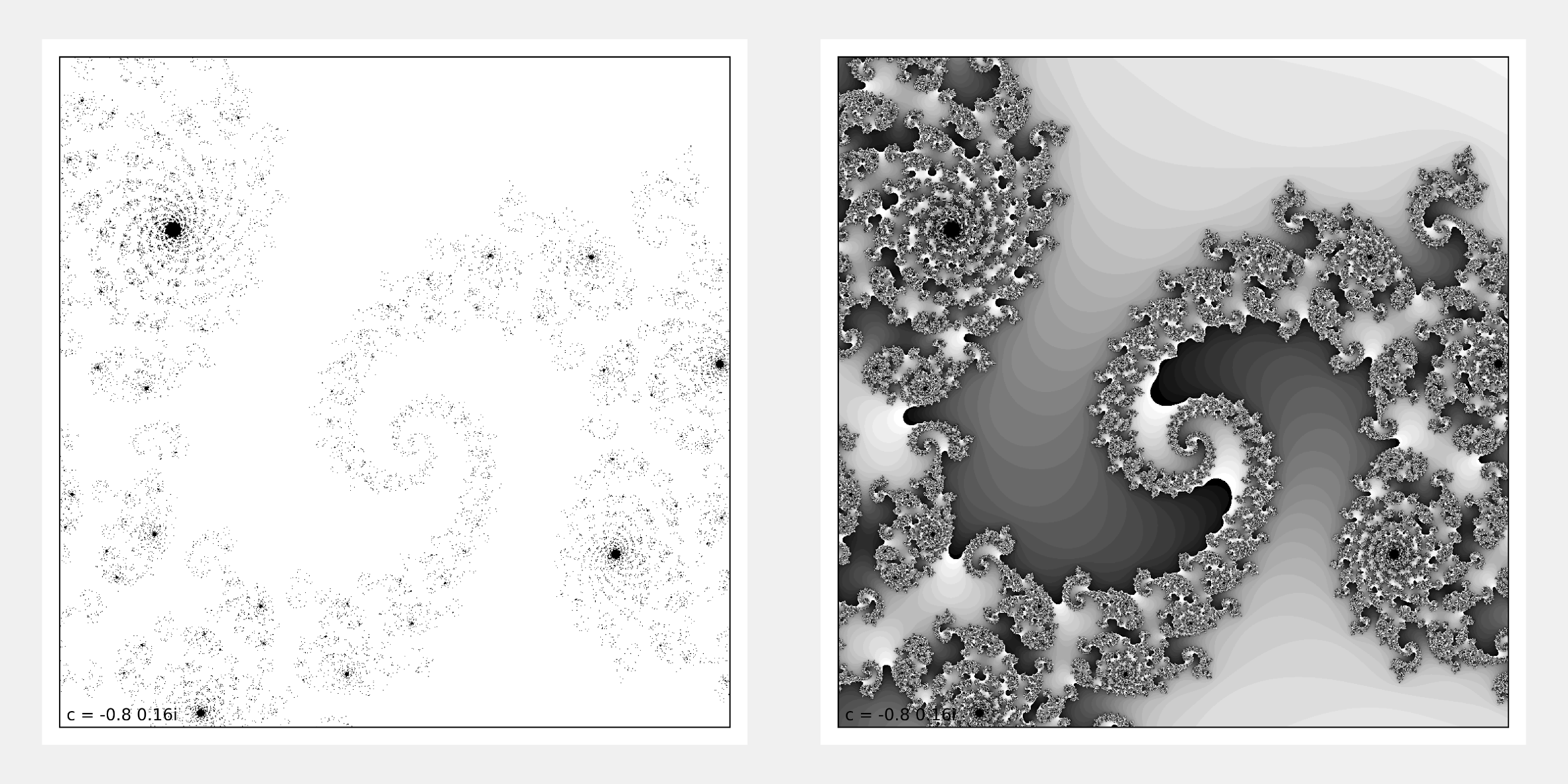
The image on the left is not too bad, but only because the collection of tiny blobs do hint at an intricate structure.
We need a new method.
Distance Estimation (by Gradient) Method
You will have noticed that away from the Mandelbrot and Julia sets, the escape-time coloured regions are larger. Their isolines are more widely spaced out. Closer to the boundary, the regions are thinner, the isolines are pressed more closely together. The following image highlights these isolines.

If you are familiar with topographic maps, you'll know that altitude (height) isolines close together means a steeper rise or fall, and widely spaced isolines means a shallow rise or descent. The same is true here.
The gradient of the magnitude of $z$ closer to the edge is higher than the gradient further away from the edge.

This is the key realisation that is behind the Distance Estimation Method. It uses the gradient to estimate the distance from the boundary (any boundary) of the Mandelbrot or Julia sets.
The benefit of this method is that the points we test, the points that correspond to the grid of pixels, only need to be near the edge of the Mandelbrot or Julia sets to detect that edge. For very fine filaments, again, the points only need to be near them to detect them.
Results!
Further below, we'll talk about the algorithm and necessary calculations, but for now let's see how this method improves on the above Mandelbrot and Julia zooms.
The following shows the exact same zoom into the Mandelbrot set as above. The newly revealed structure is very impressive!


The Algorithm
Before we write down the algorithm, let's first derive how the gradient is calculated.
The primary calculation is the iteration:
$$z_{n+1} = z_n^2 + c$$
For the Mandelbrot set, $z_0=0$ and $c$ is the point being tested. For Julia sets, $c$ is fixed, and $z_0$ is the point being tested.
Now let's work out the gradient (with thanks to Claude for helpful guidance on math stackexchange).
For the Julia set, we have fixed $c$ and are testing each $z_0$. Therefore the gradient of $z_n$ is with respect to $z_0$.
We can differentiate the primary iteration expression using the chain rule, noting that $c$ is constant so its differential is zero.
$$ \frac{d}{dz_0} z_{n+1} = 2 \times z_n \times \frac{d}{dz_0} z_{n} + 0$$
We can write this more simply as
$$z_{n+1}' = 2 z_n z_n'$$
Whilst this may look unhelpful, this form actually works well with the iterative algorithm. That is, at each iteration:
- as usual, we calculate $z_{n+1}$ from the previous $z_n$ using $z_{n+1} = z_n^2 + c$
- we also calculate $z_{n+1}'$ from the previous $z_n'$ using $z_{n+1}' = 2 z_n z_n'$
But what should the initial value of the gradient $z_0'$ be set to? Well,
$$z_0' = \frac{dz_0}{dz_0} = 1$$
This tell us to initialise $z_0'$ to 1, in the case of Julia sets.
For the Mandelbrot set, we have fixed $z_0 = 0$ and are testing different $c$. Therefore the gradient of $z_n$ is with respect to $c$.
The differentiation is slightly different now.
$$ \frac{d}{dc} z_{n+1} = 2 \times z_n \times \frac{d}{dc} z_{n} + 1$$
We can write this more simply as
$$z_{n+1}' = 2 z_n z_n' + 1$$
Again, what should the initial value of the gradient $z_0'$ be set to? This time,
$$z_0' = \frac{dz_0}{dc} = 0$$
So we initialise $z_0'$ to 0, in the case of the Mandelbrot set.
DEM Mandelbrot Set Pseudocode
- or each test point, calculate $c$
- initialise $z_{0}=(0+0i)$
- also initialise the gradient $dz_{0}=(0+0i)$
- for the maximum allowed iterations
- calculate next $z$ using $z\mapsto z^{2}+c$
- calculate next gradient $dz$ using $dz\mapsto2\cdot z\cdot dz+1$
- break out of iteration loop if $|z|>4$ escape condition met
- calculate the distance estimate as $d=\left(|z|\cdot\log|z|\right)/|dz|$
- colour the pixel based on distance estimate, for example $255\times\tanh(d\times\text{resolution}/\text{size})$
Because we're primarily using this technique to explore fine detail, we'll boost the maximum allowed iterations to 4096. We'll also increase the escape radius from 2 to 4, to give the gradient a chance to develop. Both of these will cause the rendering to take longer.
The suggestion for colouring the pixel uses the hyperbolic tangent $\tanh()$ function which squishes all values, no matter how large, into the range 0 to 1, ready for scaling up to 0-255.
Notice that the pixel colour is not based on escape speed, the iterations it took to meet the escape condition, but the distance estimate, which itself is based on the gradient of the orbit of $z$.
The distance estime $d=\left(|z|\cdot\log|z|\right)/|dz|$ is the only thing we haven't explained here. Your can find out more here. The key is that the larger the gradient the smaller the distance, the rest is scaling.
DEM Julia Set Pseudocode
The algorithm changes slightly for Julia sets.
- $c$ is chosen and fixed
- for each test point, calculate $z_{0}$
- also initialise the gradient $dz_{0}=(1+0i)$
- for the maximum allowed iterations
- calculate next $z$ using $z\mapsto z^{2}+c$
- calculate next gradient $dz$ using $dz\mapsto2\cdot z\cdot dz$
- break out of iteration loop if $|z|>4$ escape condition met
- calculate the distance estimate as $d=\left(|z|\cdot\log|z|\right)/|dz|$
- colour the pixel based on distance estimate, for example $255\times\tanh(d\times\text{resolution}/\text{size})$
Notice the gradient is initialised to 1, not 0, and is updated as $dz\mapsto2\cdot z\cdot dz$, not $dz\mapsto2\cdot z\cdot dz+1$.
Art
The following is a zoom into the Mandelbtot set rendered using this Distance Estimation method.

I love the different shapes and balance of positive and negative space, and also the contrast between the spiral and patterned regions.
I love it so much, I made it the cover image of the Second Edition of Make Your Own Mandelbrot !